from factor graph draw polar code tree gai sarkis stimming

Factor Graphs and GTSAM

This is an updated version of the 2012 tech-report Factor Graphs and GTSAM: A Hands-on Introduction by Frank Dellaert. A more thorough introduction to the use of factor graphs in robotics is the 2017 article Factor graphs for robot perception by Frank Dellaert and Michael Kaess.

Overview

Factor graphs are graphical models (, 2009) that are well suited to modeling complex estimation problems, such as Simultaneous Localization and Mapping (SLAM) or Structure from Motion (SFM). You might be familiar with another often used graphical model, Bayes networks, which are directed acyclic graphs. A factor graph, however, is a bipartite graph consisting of factors connected to variables. The variables represent the unknown random variables in the estimation problem, whereas the factors represent probabilistic constraints on those variables, derived from measurements or prior knowledge. In the following sections I will illustrate this with examples from both robotics and vision.

The GTSAM toolbox (GTSAM stands for "Georgia Tech Smoothing and Mapping") toolbox is a BSD-licensed C++ library based on factor graphs, developed at the Georgia Institute of Technology by myself, many of my students, and collaborators. It provides state of the art solutions to the SLAM and SFM problems, but can also be used to model and solve both simpler and more complex estimation problems. It also provides a MATLAB interface which allows for rapid prototype development, visualization, and user interaction.

GTSAM exploits sparsity to be computationally efficient. Typically measurements only provide information on the relationship between a handful of variables, and hence the resulting factor graph will be sparsely connected. This is exploited by the algorithms implemented in GTSAM to reduce computational complexity. Even when graphs are too dense to be handled efficiently by direct methods, GTSAM provides iterative methods that are quite efficient regardless.

You can download the latest version of GTSAM from our Github repo.

Table of Contents

1 Factor Graphs

Let us start with a one-page primer on factor graphs, which in no way replaces the excellent and detailed reviews by Kschischang et al. (2001) and Loeliger (2004).

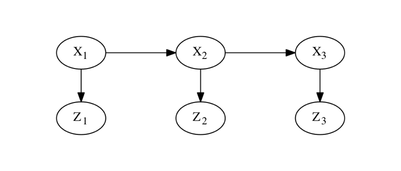Figure 1: An HMM, unrolled over three time-steps, represented by a Bayes net.

Figure 1 shows the Bayes network for a hidden Markov model (HMM) over three time steps. In a Bayes net, each node is associated with a conditional density: the top Markov chain encodes the prior

$P\left(X_1\right)$

and transition probabilities

$P\left(X_2|X_1\right)$

and

$P\left(X_3|X_2\right)$

, whereas measurements

$Z_t$

depend only on the state

$X_t$

, modeled by conditional densities

$P\left(Z_t|X_t\right)$

. Given known measurements

$z_1$

,

$z_2$

and

$z_3$

we are interested in the hidden state sequence

$\left(X_1,X_2,X_3\right)$

that maximizes the posterior probability

$P\left(X_1,X_2,X_3|Z_1=z_1,Z_2=z_2,Z_3=z_3\right)$

. Since the measurements

$Z_1$

,

$Z_2$

, and

$Z_3$

are known, the posterior is proportional to the product of six factors, three of which derive from the the Markov chain, and three likelihood factors defined as

$L\left(X_t;z\right)\propto P\left(Z_t=z|X_t\right)$

:

$$P\left(X_1,X_2,X_3|Z_1,Z_2,Z_3\right)\propto P\left(X_1\right)P\left(X_2|X_1\right)P\left(X_3|X_2\right)L\left(X_1;z_1\right)L\left(X_2;z_2\right)L\left(X_3;z_3\right)$$

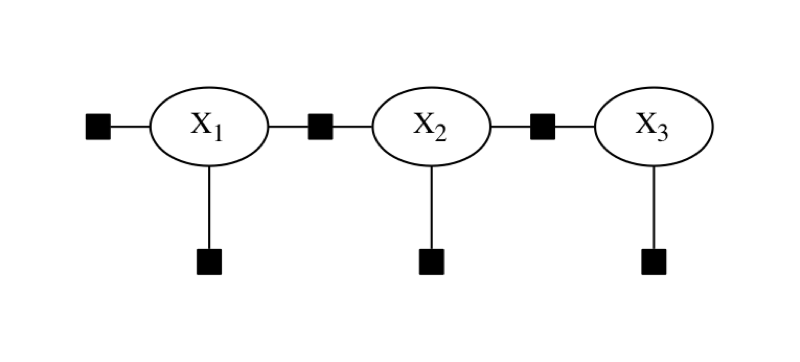Figure 2: An HMM with observed measurements, unrolled over time, represented as a factor graph.

This motivates a different graphical model, a factor graph, in which we only represent the unknown variables

$X_1$

,

$X_2$

, and

$X_3$

, connected to factors that encode probabilistic information on them, as in Figure 2. To do maximum a-posteriori (MAP) inference, we then maximize the product

$$f\left(X_1,X_2,X_3\right)=\prod f_i\left(X_i\right)$$

i.e., the value of the factor graph. It should be clear from the figure that the connectivity of a factor graph encodes, for each factor

$f_i$

, which subset of variables

$X_i$

it depends on. In the examples below, we use factor graphs to model more complex MAP inference problems in robotics.

2 Modeling Robot Motion

2.1 Modeling with Factor Graphs

Before diving into a SLAM example, let us consider the simpler problem of modeling robot motion. This can be done with a continuous Markov chain, and provides a gentle introduction to GTSAM.

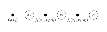Figure 3: Factor graph for robot localization.

The factor graph for a simple example is shown in Figure 3. There are three variables

$x_1$

,

$x_2$

, and

$x_3$

which represent the poses of the robot over time, rendered in the figure by the open-circle variable nodes. In this example, we have one unary factor

$f_0\left(x_1\right)$

on the first pose

$x_1$

that encodes our prior knowledge about

$x_1$

, and two binary factors that relate successive poses, respectively

$f_1\left(x_1,x_2;o_1\right)$

and

$f_2\left(x_2,x_3;o_2\right)$

, where

$o_1$

and

$o_2$

represent odometry measurements.

2.2 Creating a Factor Graph

The following C++ code, included in GTSAM as an example, creates the factor graph in Figure 3:

// Create an empty nonlinear factor graph NonlinearFactorGraph graph;  // Add a Gaussian prior on pose x_1 Pose2 priorMean(0.0, 0.0, 0.0); noiseModel::Diagonal::shared_ptr priorNoise =   noiseModel::Diagonal::Sigmas(Vector3(0.3, 0.3, 0.1)); graph.add(PriorFactor<Pose2>(1, priorMean, priorNoise));  // Add two odometry factors Pose2 odometry(2.0, 0.0, 0.0); noiseModel::Diagonal::shared_ptr odometryNoise =   noiseModel::Diagonal::Sigmas(Vector3(0.2, 0.2, 0.1)); graph.add(BetweenFactor<Pose2>(1, 2, odometry, odometryNoise)); graph.add(BetweenFactor<Pose2>(2, 3, odometry, odometryNoise));              

Above, line 2 creates an empty factor graph. We then add the factor

$f_0\left(x_1\right)$

on lines 5-8 as an instance of PriorFactor<T> , a templated class provided in the slam subfolder, with T=Pose2 . Its constructor takes a variable Key (in this case 1), a mean of type Pose2, created on Line 5, and a noise model for the prior density. We provide a diagonal Gaussian of type noiseModel::Diagonal by specifying three standard deviations in line 7, respectively 30 cm. on the robot's position, and 0.1 radians on the robot's orientation. Note that the Sigmas constructor returns a shared pointer, anticipating that typically the same noise models are used for many different factors.

Similarly, odometry measurements are specified as Pose2 on line 11, with a slightly different noise model defined on line 12-13. We then add the two factors

$f_1\left(x_1,x_2;o_1\right)$

and

$f_2\left(x_2,x_3;o_2\right)$

on lines 14-15, as instances of yet another templated class, BetweenFactor<T> , again with T=Pose2 .

When running the example (make OdometryExample.run on the command prompt), it will print out the factor graph as follows:

Factor Graph: size: 3 Factor 0: PriorFactor on 1   prior mean: (0, 0, 0)   noise model: diagonal sigmas [0.3; 0.3; 0.1]; Factor 1: BetweenFactor(1,2)   measured: (2, 0, 0)   noise model: diagonal sigmas [0.2; 0.2; 0.1]; Factor 2: BetweenFactor(2,3)   measured: (2, 0, 0)   noise model: diagonal sigmas [0.2; 0.2; 0.1];              

2.3 Factor Graphs versus Values

At this point it is instructive to emphasize two important design ideas underlying GTSAM:

1. The factor graph and its embodiment in code specify the joint probability distribution $P\left(X|Z\right)$ over the entire trajectory $X=\left\{x_1,x_2,x_3\right\}$ of the robot, rather than just the last pose. This smoothing view of the world gives GTSAM its name: "smoothing and mapping". Later in this document we will talk about how we can also use GTSAM to do filtering (which you often do not want to do) or incremental inference (which we do all the time).
2. A factor graph in GTSAM is just the specification of the probability density $P\left(X|Z\right)$, and the corresponding FactorGraph class and its derived classes do not ever contain a "solution". Rather, there is a separate type Values that is used to specify specific values for (in this case) $x_1$, $x_2$, and $x_3$, which can then be used to evaluate the probability (or, more commonly, the error) associated with particular values.

The latter point is often a point of confusion with beginning users of GTSAM. It helps to remember that when designing GTSAM we took a functional approach of classes corresponding to mathematical objects, which are usually immutable. You should think of a factor graph as a function to be applied to values -as the notation

$f\left(X\right)\propto P\left(X|Z\right)$

implies- rather than as an object to be modified.

2.4 Non-linear Optimization in GTSAM

The listing below creates a Values instance, and uses it as the initial estimate to find the maximum a-posteriori (MAP) assignment for the trajectory

$X$

:

// create (deliberately inaccurate) initial estimate Values initial; initial.insert(1, Pose2(0.5, 0.0, 0.2)); initial.insert(2, Pose2(2.3, 0.1, -0.2)); initial.insert(3, Pose2(4.1, 0.1, 0.1));  // optimize using Levenberg-Marquardt optimization Values result = LevenbergMarquardtOptimizer(graph, initial).optimize();              

Lines 2-5 in Listing 2.4 create the initial estimate, and on line 8 we create a non-linear Levenberg-Marquardt style optimizer, and call optimize using default parameter settings. The reason why GTSAM needs to perform non-linear optimization is because the odometry factors

$f_1\left(x_1,x_2;o_1\right)$

and

$f_2\left(x_2,x_3;o_2\right)$

are non-linear, as they involve the orientation of the robot. This also explains why the factor graph we created in Listing 2.2 is of type NonlinearFactorGraph . The optimization class linearizes this graph, possibly multiple times, to minimize the non-linear squared error specified by the factors.

The relevant output from running the example is as follows:

Initial Estimate: Values with 3 values: Value 1: (0.5, 0, 0.2) Value 2: (2.3, 0.1, -0.2) Value 3: (4.1, 0.1, 0.1)  Final Result: Values with 3 values: Value 1: (-1.8e-16, 8.7e-18, -9.1e-19) Value 2: (2, 7.4e-18, -2.5e-18) Value 3: (4, -1.8e-18, -3.1e-18)              

It can be seen that, subject to very small tolerance, the ground truth solution

$x_1=\left(0,0,0\right)$

,

$x_2=\left(2,0,0\right)$

, and

$x_3=\left(4,0,0\right)$

is recovered.

2.5 Full Posterior Inference

GTSAM can also be used to calculate the covariance matrix for each pose after incorporating the information from all measurements

$Z$

. Recognizing that the factor graph encodes the posterior density

$P\left(X|Z\right)$

, the mean

$\mu$

together with the covariance

$\Sigma$

for each pose

$x$

approximate the marginal posterior density

$P\left(x|Z\right)$

. Note that this is just an approximation, as even in this simple case the odometry factors are actually non-linear in their arguments, and GTSAM only computes a Gaussian approximation to the true underlying posterior.

The following C++ code will recover the posterior marginals:

// Query the marginals cout.precision(2); Marginals marginals(graph, result); cout << "x1 covariance:\n" << marginals.marginalCovariance(1) << endl; cout << "x2 covariance:\n" << marginals.marginalCovariance(2) << endl; cout << "x3 covariance:\n" << marginals.marginalCovariance(3) << endl;              

The relevant output from running the example is as follows:

x1 covariance:        0.09     1.1e-47     5.7e-33     1.1e-47        0.09     1.9e-17     5.7e-33     1.9e-17        0.01 x2 covariance:        0.13     4.7e-18     2.4e-18     4.7e-18        0.17        0.02     2.4e-18        0.02        0.02 x3 covariance:        0.17     2.7e-17     8.4e-18     2.7e-17        0.37        0.06     8.4e-18        0.06        0.03              

What we see is that the marginal covariance

$P\left(x_1|Z\right)$

on

$x_1$

is simply the prior knowledge on

$x_1$

, but as the robot moves the uncertainty in all dimensions grows without bound, and the

$y$

and

$\theta$

components of the pose become (positively) correlated.

An important fact to note when interpreting these numbers is that covariance matrices are given in relative coordinates, not absolute coordinates. This is because internally GTSAM optimizes for a change with respect to a linearization point, as do all nonlinear optimization libraries.

3 Robot Localization

3.1 Unary Measurement Factors

In this section we add measurements to the factor graph that will help us actually localize the robot over time. The example also serves as a tutorial on creating new factor types.

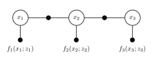Figure 4: Robot localization factor graph with unary measurement factors at each time step.

In particular, we use unary measurement factors to handle external measurements. The example from Section 2 is not very useful on a real robot, because it only contains factors corresponding to odometry measurements. These are imperfect and will lead to quickly accumulating uncertainty on the last robot pose, at least in the absence of any external measurements (see Section 2.5). Figure 4 shows a new factor graph where the prior

$f_0\left(x_1\right)$

is omitted and instead we added three unary factors

$f_1\left(x_1;z_1\right)$

,

$f_2\left(x_2;z_2\right)$

, and

$f_3\left(x_3;z_3\right)$

, one for each localization measurement

$z_t$

, respectively. Such unary factors are applicable for measurements

$z_t$

that depend only on the current robot pose, e.g., GPS readings, correlation of a laser range-finder in a pre-existing map, or indeed the presence of absence of ceiling lights (see Dellaert et al. (1999) for that amusing example).

3.2 Defining Custom Factors

In GTSAM, you can create custom unary factors by deriving a new class from the built-in class NoiseModelFactor1<T> , which implements a unary factor corresponding to a measurement likelihood with a Gaussian noise model,

$L(q;m)=\; exp\{-\frac{1}{2}{||h\left(q\right)-m||}_{\Sigma }^2\}=f\left(q\right)$

where

$m$

is the measurement,

$q$

is the unknown variable,

$h\left(q\right)$

is a (possibly nonlinear) measurement function, and

$\Sigma$

is the noise covariance. Note that

$m$

is considered known above, and the likelihood

$L\left(q;m\right)$

will only ever be evaluated as a function of

$q$

, which explains why it is a unary factor

$f\left(q\right)$

. It is always the unknown variable

$q$

that is either likely or unlikely, given the measurement.

Note: many people get this backwards, often misled by the conditional density notation

$P\left(m|q\right)$

. In fact, the likelihood

$L\left(q;m\right)$

is defined as any function of

$q$

proportional to

$P\left(m|q\right)$

.

Listing 3.2 shows an example on how to define the custom factor class UnaryFactor which implements a "GPS-like" measurement likelihood:

class UnaryFactor: public NoiseModelFactor1<Pose2> {   double mx_, my_; ///< X and Y measurements  public:   UnaryFactor(Key j, double x, double y, const SharedNoiseModel& model):     NoiseModelFactor1<Pose2>(model, j), mx_(x), my_(y) {}    Vector evaluateError(const Pose2& q,                        boost::optional<Matrix&> H = boost::none) const   {     const Rot2& R = q.rotation();     if (H) (*H) = (gtsam::Matrix(2, 3) <<             R.c(), -R.s(), 0.0,             R.s(), R.c(), 0.0).finished();     return (Vector(2) << q.x() - mx_, q.y() - my_).finished();   } };              

In defining the derived class on line 1, we provide the template argument Pose2 to indicate the type of the variable

$q$

, whereas the measurement is stored as the instance variables mx_ and my_ , defined on line 2. The constructor on lines 5-6 simply passes on the variable key

$j$

and the noise model to the superclass, and stores the measurement values provided. The most important function to has be implemented by every factor class is evaluateError , which should return

$E\left(q\right)=h\left(q\right)-m$

which is done on line 12. Importantly, because we want to use this factor for nonlinear optimization (see e.g., Dellaert and Kaess 2006 for details), whenever the optional argument

$H$

is provided, a Matrix reference, the function should assign the Jacobian of

$h\left(q\right)$

to it, evaluated at the provided value for

$q$

. This is done for this example on line 11. In this case, the Jacobian of the 2-dimensional function

$h$

, which just returns the position of the robot,

$$h\left(q\right)=\left[\begin{array}{c}{q}_x\\ q_y\end{array}\right]$$

with respect the 3-dimensional pose

$q=\left(q_x,q_y,q_{\theta }\right)$

, yields the following

$2\times 3$

matrix:

$$H=\left[\begin{array}{ccc}cos\left(q_{\theta }\right)& -sin\left(q_{\theta }\right)& 0\\ sin\left(q_{\theta }\right)& cos\left(q_{\theta }\right)& 0\end{array}\right]$$

Important Note

Many of our users, when attempting to create a custom factor, are initially surprised at the Jacobian matrix not agreeing with their intuition. For example, above you might simply expect a

$2\times 3$

diagonal matrix. This would be true for variables belonging to a vector space. However, in GTSAM we define the Jacobian more generally to be the matrix

$H$

such that

$$h\left(q{e}^{\hat{\xi }}\right)\approx h\left(q\right)+H\xi$$

where

$\xi =\left(\delta x,\delta y,\delta \theta \right)$

is an incremental update and

$exp\hat{\xi }$

is the exponential map for the variable we want to update, In this case

$q\in SE\left(2\right)$

, where

$SE\left(2\right)$

is the group of 2D rigid transforms, implemented by Pose2 . The exponential map for

$SE\left(2\right)$

can be approximated to first order as

$$exp\hat{\xi }\approx \left[\begin{array}{ccc}1& -\delta \theta & \delta x\\ \delta \theta & 1& \delta x\\ 0& 0& 1\end{array}\right]$$

when using the

$3\times 3$

matrix representation for 2D poses, and hence

$$h\left(q{e}^{\hat{\xi }}\right)\approx h\left(\left[\begin{array}{ccc}cos\left(q_{\theta }\right)& -sin\left(q_{\theta }\right)& q_x\\ sin\left(q_{\theta }\right)& cos\left(q_{\theta }\right)& q_y\\ 0& 0& 1\end{array}\right]\left[\begin{array}{ccc}1& -\delta \theta & \delta x\\ \delta \theta & 1& \delta x\\ 0& 0& 1\end{array}\right]\right)=\left[\begin{array}{c}{q}_x+cos\left(q_{\theta }\right)\delta x-sin\left(q_{\theta }\right)\delta y\\ q_y+sin\left(q_{\theta }\right)\delta x+cos\left(q_{\theta }\right)\delta y\end{array}\right]$$

which then explains the Jacobian

$H$

.

3.3 Using Custom Factors

The following C++ code fragment illustrates how to create and add custom factors to a factor graph:

// add unary measurement factors, like GPS, on all three poses noiseModel::Diagonal::shared_ptr unaryNoise =  noiseModel::Diagonal::Sigmas(Vector2(0.1, 0.1)); // 10cm std on x,y graph.add(boost::make_shared<UnaryFactor>(1, 0.0, 0.0, unaryNoise)); graph.add(boost::make_shared<UnaryFactor>(2, 2.0, 0.0, unaryNoise)); graph.add(boost::make_shared<UnaryFactor>(3, 4.0, 0.0, unaryNoise));              

In Listing 3.3, we create the noise model on line 2-3, which now specifies two standard deviations on the measurements

$m_x$

and

$m_y$

. On lines 4-6 we create shared_ptr versions of three newly created UnaryFactor instances, and add them to graph. GTSAM uses shared pointers to refer to factors in factor graphs, and boost::make_shared is a convenience function to simultaneously construct a class and create a shared_ptr to it. We obtain the factor graph from Figure 4.

3.4 Full Posterior Inference

The three GPS factors are enough to fully constrain all unknown poses and tie them to a "global" reference frame, including the three unknown orientations. If not, GTSAM would have exited with a singular matrix exception. The marginals can be recovered exactly as in Section 2.5, and the solution and marginal covariances are now given by the following:

Final Result: Values with 3 values: Value 1: (-1.5e-14, 1.3e-15, -1.4e-16) Value 2: (2, 3.1e-16, -8.5e-17) Value 3: (4, -6e-16, -8.2e-17)  x1 covariance:       0.0083      4.3e-19     -1.1e-18      4.3e-19       0.0094      -0.0031     -1.1e-18      -0.0031       0.0082 x2 covariance:       0.0071      2.5e-19     -3.4e-19      2.5e-19       0.0078      -0.0011     -3.4e-19      -0.0011       0.0082 x3 covariance:      0.0083     4.4e-19     1.2e-18     4.4e-19      0.0094      0.0031     1.2e-18      0.0031       0.018            

Comparing this with the covariance matrices in Section 2.5, we can see that the uncertainty no longer grows without bounds as measurement uncertainty accumulates. Instead, the "GPS" measurements more or less constrain the poses evenly, as expected.

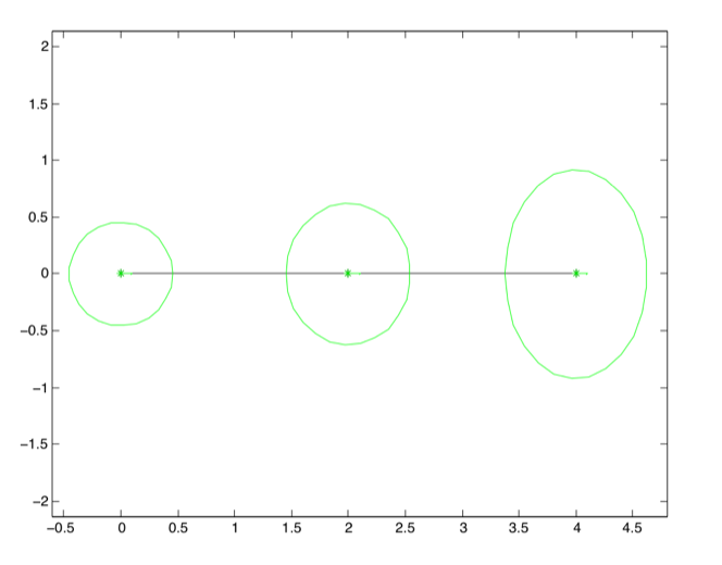
Sub-Figure a: Odometry marginals

Figure 5: Comparing the marginals resulting from the "odometry" factor graph in Figure 3 and the "localization" factor graph in Figure 4.

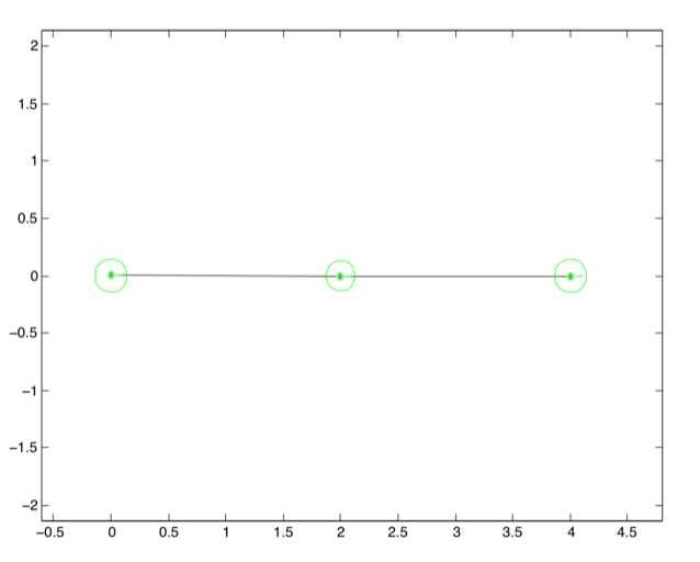
Sub-Figure b: Localization Marginals

It helps a lot when we view this graphically, as in Figure 5, where I show the marginals on position as 5-sigma covariance ellipses that contain 99.9996% of all probability mass. For the odometry marginals, it is immediately apparent from the figure that (1) the uncertainty on pose keeps growing, and (2) the uncertainty on angular odometry translates into increasing uncertainty on y. The localization marginals, in contrast, are constrained by the unary factors and are all much smaller. In addition, while less apparent, the uncertainty on the middle pose is actually smaller as it is constrained by odometry from two sides.

You might now be wondering how we produced these figures. The answer is via the MATLAB interface of GTSAM, which we will demonstrate in the next section.

4 PoseSLAM

4.1 Loop Closure Constraints

The simplest instantiation of a SLAM problem is PoseSLAM, which avoids building an explicit map of the environment. The goal of SLAM is to simultaneously localize a robot and map the environment given incoming sensor measurements (Durrant-Whyte and Bailey, 2006). Besides wheel odometry, one of the most popular sensors for robots moving on a plane is a 2D laser-range finder, which provides both odometry constraints between successive poses, and loop-closure constraints when the robot re-visits a previously explored part of the environment.

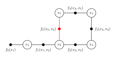Figure 6: Factor graph for PoseSLAM.

A factor graph example for PoseSLAM is shown in Figure 6. The following C++ code, included in GTSAM as an example, creates this factor graph in code:

NonlinearFactorGraph graph; noiseModel::Diagonal::shared_ptr priorNoise =   noiseModel::Diagonal::Sigmas(Vector3(0.3, 0.3, 0.1)); graph.add(PriorFactor<Pose2>(1, Pose2(0, 0, 0), priorNoise));  // Add odometry factors noiseModel::Diagonal::shared_ptr model =   noiseModel::Diagonal::Sigmas(Vector3(0.2, 0.2, 0.1)); graph.add(BetweenFactor<Pose2>(1, 2, Pose2(2, 0, 0     ), model)); graph.add(BetweenFactor<Pose2>(2, 3, Pose2(2, 0, M_PI_2), model)); graph.add(BetweenFactor<Pose2>(3, 4, Pose2(2, 0, M_PI_2), model)); graph.add(BetweenFactor<Pose2>(4, 5, Pose2(2, 0, M_PI_2), model));  // Add the loop closure constraint graph.add(BetweenFactor<Pose2>(5, 2, Pose2(2, 0, M_PI_2), model));            

As before, lines 1-4 create a nonlinear factor graph and add the unary factor

$f_0\left(x_1\right)$

. As the robot travels through the world, it creates binary factors

$f_t\left(x_t,x_{t+1}\right)$

corresponding to odometry, added to the graph in lines 6-12 (Note that M_PI_2 refers to pi/2). But line 15 models a different event: a loop closure. For example, the robot might recognize the same location using vision or a laser range finder, and calculate the geometric pose constraint to when it first visited this location. This is illustrated for poses

$x_5$

and

$x_2$

, and generates the (red) loop closing factor

$f_5\left(x_5,x_2\right)$

.

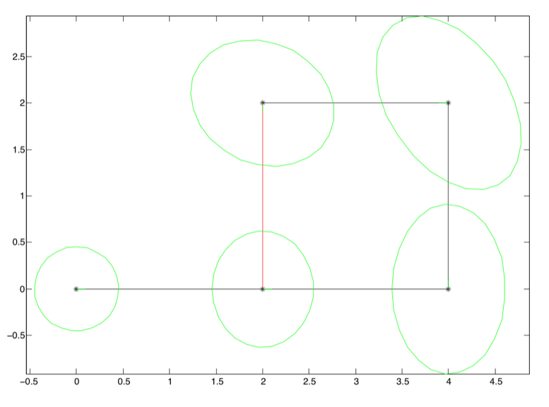Figure 7: The result of running optimize on the factor graph in Figure 6.

We can optimize this factor graph as before, by creating an initial estimate of type Values , and creating and running an optimizer. The result is shown graphically in Figure 7, along with covariance ellipses shown in green. These 5-sigma covariance ellipses in 2D indicate the marginal over position, over all possible orientations, and show the area which contain 99.9996% of the probability mass. The graph shows in a clear manner that the uncertainty on pose

$x_5$

is now much less than if there would be only odometry measurements. The pose with the highest uncertainty,

$x_4$

, is the one furthest away from the unary constraint

$f_0\left(x_1\right)$

, which is the only factor tying the graph to a global coordinate frame.

The figure above was created using an interface that allows you to use GTSAM from within MATLAB, which provides for visualization and rapid development. We discuss this next.

4.2 Using the MATLAB Interface

A large subset of the GTSAM functionality can be accessed through wrapped classes from within MATLAB

. The following code excerpt is the MATLAB equivalent of the C++ code in Listing 4.1:

graph = NonlinearFactorGraph; priorNoise = noiseModel.Diagonal.Sigmas([0.3; 0.3; 0.1]); graph.add(PriorFactorPose2(1, Pose2(0, 0, 0), priorNoise));  %% Add odometry factors model = noiseModel.Diagonal.Sigmas([0.2; 0.2; 0.1]); graph.add(BetweenFactorPose2(1, 2, Pose2(2, 0, 0   ), model)); graph.add(BetweenFactorPose2(2, 3, Pose2(2, 0, pi/2), model)); graph.add(BetweenFactorPose2(3, 4, Pose2(2, 0, pi/2), model)); graph.add(BetweenFactorPose2(4, 5, Pose2(2, 0, pi/2), model));  %% Add pose constraint graph.add(BetweenFactorPose2(5, 2, Pose2(2, 0, pi/2), model));            

Note that the code is almost identical, although there are a few syntax and naming differences:

• Objects are created by calling a constructor instead of allocating them on the heap.
• Namespaces are done using dot notation, i.e., noiseModel::Diagonal::SigmasClasses becomes noiseModel.Diagonal.Sigmas .
• Vector and Matrix classes in C++ are just vectors/matrices in MATLAB.
• As templated classes do not exist in MATLAB, these have been hardcoded in the GTSAM interface, e.g., PriorFactorPose2 corresponds to the C++ class PriorFactor<Pose2> , etc.

After executing the code, you can call whos on the MATLAB command prompt to see the objects created. Note that the indicated Class corresponds to the wrapped C++ classes:

>> whos   Name                 Size            Bytes  Class   graph                1x1               112  gtsam.NonlinearFactorGraph   priorNoise           1x1               112  gtsam.noiseModel.Diagonal   model                1x1               112  gtsam.noiseModel.Diagonal   initialEstimate      1x1               112  gtsam.Values   optimizer            1x1               112  gtsam.LevenbergMarquardtOptimizer            

In addition, any GTSAM object can be examined in detail, yielding identical output to C++:

>> priorNoise diagonal sigmas [0.3; 0.3; 0.1];  >> graph size: 6 factor 0: PriorFactor on 1   prior mean: (0, 0, 0)   noise model: diagonal sigmas [0.3; 0.3; 0.1]; factor 1: BetweenFactor(1,2)   measured: (2, 0, 0)   noise model: diagonal sigmas [0.2; 0.2; 0.1]; factor 2: BetweenFactor(2,3)   measured: (2, 0, 1.6)   noise model: diagonal sigmas [0.2; 0.2; 0.1]; factor 3: BetweenFactor(3,4)   measured: (2, 0, 1.6)   noise model: diagonal sigmas [0.2; 0.2; 0.1]; factor 4: BetweenFactor(4,5)   measured: (2, 0, 1.6)   noise model: diagonal sigmas [0.2; 0.2; 0.1]; factor 5: BetweenFactor(5,2)   measured: (2, 0, 1.6)   noise model: diagonal sigmas [0.2; 0.2; 0.1];            

And it does not stop there: we can also call some of the functions defined for factor graphs. E.g.,

>> graph.error(initialEstimate) ans =    20.1086  >> graph.error(result) ans =    8.2631e-18            

computes the sum-squared error $\frac{1}{2}\sum _i{||h_i\left(X_i\right)-z_i||}_{\Sigma }^2$ before and after optimization.

4.3 Reading and Optimizing Pose Graphs

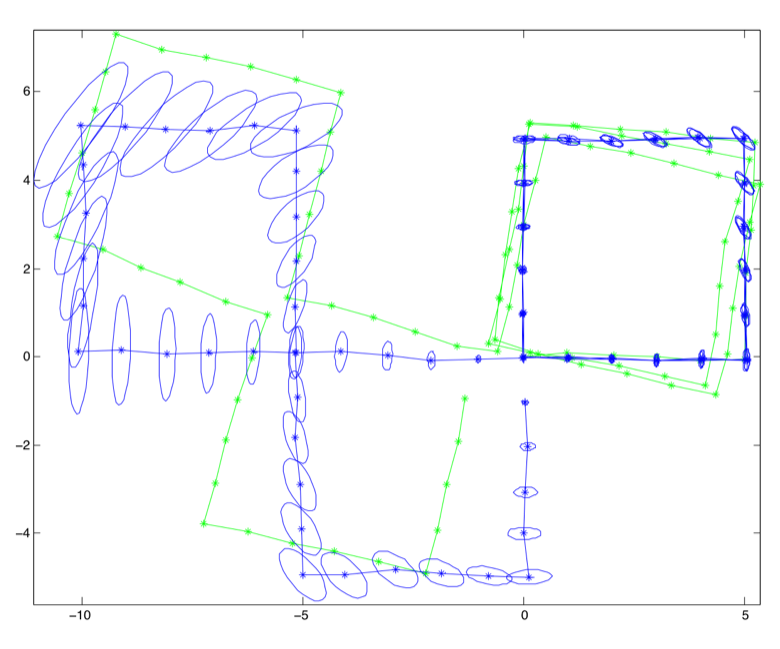Figure 8: MATLAB plot of small Manhattan world example with 100 poses (due to Ed Olson). The initial estimate is shown in green. The optimized trajectory, with covariance ellipses, in blue.

The ability to work in MATLAB adds a much quicker development cycle, and effortless graphical output. The optimized trajectory in Figure 8 was produced by the code below, in which load2D reads TORO files. To see how plotting is done, refer to the full source code.

%% Initialize graph, initial estimate, and odometry noise datafile = findExampleDataFile('w100.graph'); model = noiseModel.Diagonal.Sigmas([0.05; 0.05; 5*pi/180]); [graph,initial] = load2D(datafile, model);  %% Add a Gaussian prior on pose x_0 priorMean = Pose2(0, 0, 0); priorNoise = noiseModel.Diagonal.Sigmas([0.01; 0.01; 0.01]); graph.add(PriorFactorPose2(0, priorMean, priorNoise));  %% Optimize using Levenberg-Marquardt optimization and get marginals optimizer = LevenbergMarquardtOptimizer(graph, initial); result = optimizer.optimizeSafely; marginals = Marginals(graph, result);            

4.4 PoseSLAM in 3D

PoseSLAM can easily be extended to 3D poses, but some care is needed to update 3D rotations. GTSAM supports both quaternions and

$3\times 3$

rotation matrices to represent 3D rotations. The selection is made via the compile flag GTSAM_USE_QUATERNIONS.

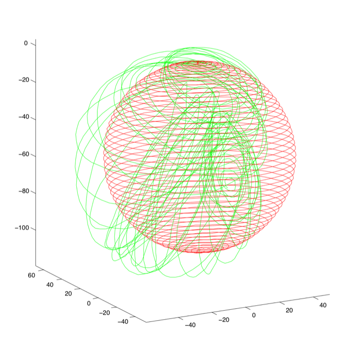Figure 9: 3D plot of sphere example (due to Michael Kaess). The very wrong initial estimate, derived from odometry, is shown in green. The optimized trajectory is shown red. Code below:

%% Initialize graph, initial estimate, and odometry noise datafile = findExampleDataFile('sphere2500.txt'); model = noiseModel.Diagonal.Sigmas([5*pi/180; 5*pi/180; 5*pi/180; 0.05; 0.05; 0.05]); [graph,initial] = load3D(datafile, model, true, 2500); plot3DTrajectory(initial, 'g-', false); % Plot Initial Estimate  %% Read again, now with all constraints, and optimize graph = load3D(datafile, model, false, 2500); graph.add(NonlinearEqualityPose3(0, initial.atPose3(0))); optimizer = LevenbergMarquardtOptimizer(graph, initial); result = optimizer.optimizeSafely(); plot3DTrajectory(result, 'r-', false); axis equal;            

5 Landmark-based SLAM

5.1 Basics

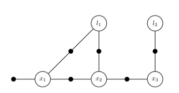Figure 10: Factor graph for landmark-based SLAM

In landmark-based SLAM, we explicitly build a map with the location of observed landmarks, which introduces a second type of variable in the factor graph besides robot poses. An example factor graph for a landmark-based SLAM example is shown in Figure 10, which shows the typical connectivity: poses are connected in an odometry Markov chain, and landmarks are observed from multiple poses, inducing binary factors. In addition, the pose

$x_1$

has the usual prior on it.

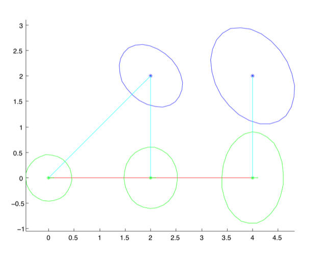Figure 11: The optimized result along with covariance ellipses for both poses (in green) and landmarks (in blue). Also shown are the trajectory (red) and landmark sightings (cyan).

The factor graph from Figure 10 can be created using the MATLAB code in Listing 5.1. As before, on line 2 we create the factor graph, and Lines 8-18 create the prior/odometry chain we are now familiar with. However, the code on lines 20-25 is new: it creates three measurement factors, in this case "bearing/range" measurements from the pose to the landmark.

% Create graph container and add factors to it graph = NonlinearFactorGraph;  % Create keys for variables i1 = symbol('x',1); i2 = symbol('x',2); i3 = symbol('x',3); j1 = symbol('l',1); j2 = symbol('l',2);  % Add prior priorMean = Pose2(0.0, 0.0, 0.0); % prior at origin priorNoise = noiseModel.Diagonal.Sigmas([0.3; 0.3; 0.1]); % add directly to graph graph.add(PriorFactorPose2(i1, priorMean, priorNoise));  % Add odometry odometry = Pose2(2.0, 0.0, 0.0); odometryNoise = noiseModel.Diagonal.Sigmas([0.2; 0.2; 0.1]); graph.add(BetweenFactorPose2(i1, i2, odometry, odometryNoise)); graph.add(BetweenFactorPose2(i2, i3, odometry, odometryNoise));  % Add bearing/range measurement factors degrees = pi/180; brNoise = noiseModel.Diagonal.Sigmas([0.1; 0.2]); graph.add(BearingRangeFactor2D(i1, j1, Rot2(45*degrees), sqrt(8), brNoise)); graph.add(BearingRangeFactor2D(i2, j1, Rot2(90*degrees), 2, brNoise)); graph.add(BearingRangeFactor2D(i3, j2, Rot2(90*degrees), 2, brNoise));            

5.2 Of Keys and Symbols

The only unexplained code is on lines 4-6: here we create integer keys for the poses and landmarks using the symbol function. In GTSAM, we address all variables using the Ke y type, which is just a typedef to size_t

. The keys do not have to be numbered continuously, but they do have to be unique within a given factor graph. For factor graphs with different types of variables, we provide the symbol function in MATLAB, and the Symbol type in C++, to help you create (large) integer keys that are far apart in the space of possible keys, so you don't have to think about starting the point numbering at some arbitrary offset. To create a a symbol key you simply provide a character and an integer index. You can use base 0 or 1, or use arbitrary indices: it does not matter. In the code above, we we use 'x' for poses, and 'l' for landmarks.

The optimized result for the factor graph created by Listing 5.1 is shown in Figure 11, and it is readily apparent that the landmark

$l_1$

with two measurements is better localized. In MATLAB we can also examine the actual numerical values, and doing so reveals some more GTSAM magic:

>> result Values with 5 values: l1: (2, 2) l2: (4, 2) x1: (-1.8e-16, 5.1e-17, -1.5e-17) x2: (2, -5.8e-16, -4.6e-16) x3: (4, -3.1e-15, -4.6e-16)

Indeed, the keys generated by symbol are automatically detected by the print method in the Values class, and rendered in human-readable form "x1", "l2", etc, rather than as large, unwieldy integers. This magic extends to most factors and other classes where the Key type is used.

5.3 A Larger Example

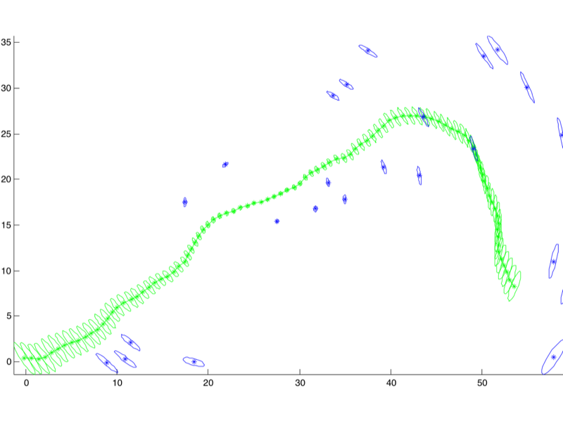Figure 12: A larger example with about 100 poses and 30 or so landmarks, as produced by gtsam_examples/PlanarSLAMExample_graph.m

GTSAM comes with a slightly larger example that is read from a .graph file by PlanarSLAMExample_graph.m, shown in Figure 12. To not clutter the figure only the marginals are shown, not the lines of sight. This example, with 119 (multivariate) variables and 517 factors optimizes in less than 10 ms.

5.4 A Real-World Example

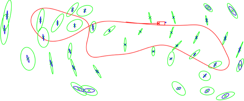Figure 13: Small section of optimized trajectory and landmarks (trees detected in a laser range finder scan) from data recorded in Sydney's Victoria Park (dataset due to Jose Guivant, U. Sydney).

A real-world example is shown in Figure 13, using data from a well known dataset collected in Sydney's Victoria Park, using a truck equipped with a laser range-finder. The covariance matrices in this figure were computed very efficiently, as explained in detail in (Kaess and Dellaert, 2009). The exact covariances (blue, smaller ellipses) obtained by our fast algorithm coincide with the exact covariances based on full inversion (orange, mostly hidden by blue). The much larger conservative covariance estimates (green, large ellipses) were based on our earlier work in (Kaess et al., 2008).

6 Structure from Motion

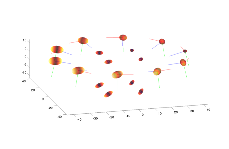Figure 14: An optimized "Structure from Motion" with 10 cameras arranged in a circle, observing the 8 vertices of a $20\times 20\times 20$ cube centered around the origin. The camera is rendered with color-coded axes, (RGB for XYZ) and the viewing direction is is along the positive Z-axis. Also shown are the 3D error covariance ellipses for both cameras and points.

Structure from Motion (SFM) is a technique to recover a 3D reconstruction of the environment from corresponding visual features in a collection of unordered images, see Figure 14. In GTSAM this is done using exactly the same factor graph framework, simply using SFM-specific measurement factors. In particular, there is a projection factor that calculates the reprojection error

$f\left(x_i,p_j;z_{ij},K\right)$

for a given camera pose

$x_i$

(a Pose3 ) and point

$p_j$

(a Point3 ). The factor is parameterized by the 2D measurement

$z_{ij}$

(a Point2 ), and known calibration parameters

$K$

(of type Cal3_S2 ). The following listing shows how to create the factor graph:

%% Add factors for all measurements noise = noiseModel.Isotropic.Sigma(2, measurementNoiseSigma); for i = 1:length(Z),      for k = 1:length(Z{i})         j = J{i}{k};         G.add(GenericProjectionFactorCal3_S2(               Z{i}{k}, noise, symbol('x', i), symbol('p', j), K));     end end            

In Listing 6, assuming that the factor graph was already created, we add measurement factors in the double loop. We loop over images with index

$i$

, and in this example the data is given as two cell arrays: Z{i} specifies a set of measurements

$z_k$

in image

$i$

, and J{i} specifies the corresponding point index. The specific factor type we use is a GenericProjectionFactorCal3_S2 , which is the MATLAB equivalent of the C++ class GenericProjectionFactor<Cal3_S2> , where Cal3_S2 is the camera calibration type we choose to use (the standard, no-radial distortion, 5 parameter calibration matrix). As before landmark-based SLAM (Section 5), here we use symbol keys except we now use the character 'p' to denote points, rather than 'l' for landmark.

Important note: a very tricky and difficult part of making SFM work is (a) data association, and (b) initialization. GTSAM does neither of these things for you: it simply provides the "bundle adjustment" optimization. In the example, we simply assume the data association is known (it is encoded in the J sets), and we initialize with the ground truth, as the intent of the example is simply to show you how to set up the optimization problem.

7 iSAM: Incremental Smoothing and Mapping

GTSAM provides an incremental inference algorithm based on a more advanced graphical model, the Bayes tree, which is kept up to date by the iSAM algorithm (incremental Smoothing and Mapping, see Kaess et al. (2008); Kaess et al. (2012) for an in-depth treatment). For mobile robots operating in real-time it is important to have access to an updated map as soon as new sensor measurements come in. iSAM keeps the map up-to-date in an efficient manner.

Listing 7 shows how to use iSAM in a simple visual SLAM example. In line 1-2 we create a NonlinearISAM object which will relinearize and reorder the variables every 3 steps. The corect value for this parameter depends on how non-linear your problem is and how close you want to be to gold-standard solution at every step. In iSAM 2.0, this parameter is not needed, as iSAM2 automatically determines when linearization is needed and for which variables.

The example involves eight 3D points that are seen from eight successive camera poses. Hence in the first step -which is omitted here- all eight landmarks and the first pose are properly initialized. In the code this is done by perturbing the known ground truth, but in a real application great care is needed to properly initialize poses and landmarks, especially in a monocular sequence.

int relinearizeInterval = 3; NonlinearISAM isam(relinearizeInterval);  // ... first frame initialization omitted ...  // Loop over the different poses, adding the observations to iSAM for (size_t i = 1; i < poses.size(); ++i) {    // Add factors for each landmark observation   NonlinearFactorGraph graph;   for (size_t j = 0; j < points.size(); ++j) {     graph.add(       GenericProjectionFactor<Pose3, Point3, Cal3_S2>         (z[i][j], noise,Symbol('x', i), Symbol('l', j), K)     );   }    // Add an initial guess for the current pose   Values initialEstimate;   initialEstimate.insert(Symbol('x', i), initial_x[i]);    // Update iSAM with the new factors   isam.update(graph, initialEstimate);  }            

The remainder of the code illustrates a typical iSAM loop:

1. Create factors for new measurements. Here, in lines 9-18, a small NonlinearFactorGraph is created to hold the new factors of type GenericProjectionFactor<Pose3, Point3, Cal3_S2> .
2. Create an initial estimate for all newly introduced variables. In this small example, all landmarks have been observed in frame 1 and hence the only new variable that needs to be initialized at each time step is the new pose. This is done in lines 20-22. Note we assume a good initial estimate is available as initial_x[i].
3. Finally, we call isam.update(), which takes the factors and initial estimates, and incrementally updates the solution, which is available through the method isam.estimate(), if desired.

8 More Applications

While a detailed discussion of all the things you can do with GTSAM will take us too far, below is a small survey of what you can expect to do, and which we did using GTSAM.

8.1 Conjugate Gradient Optimization

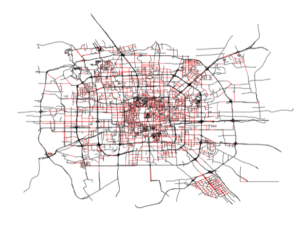Figure 15: A map of Beijing, with a spanning tree shown in black, and the remaining loop-closing constraints shown in red. A spanning tree can be used as a preconditioner by GTSAM.

GTSAM also includes efficient preconditioned conjugate gradients (PCG) methods for solving large-scale SLAM problems. While direct methods, popular in the literature, exhibit quadratic convergence and can be quite efficient for sparse problems, they typically require a lot of storage and efficient elimination orderings to be found. In contrast, iterative optimization methods only require access to the gradient and have a small memory footprint, but can suffer from poor convergence. Our method, subgraph preconditioning, explained in detail in Dellaert et al. (2010); Jian et al. (2011), combines the advantages of direct and iterative methods, by identifying a sub-problem that can be easily solved using direct methods, and solving for the remaining part using PCG. The easy sub-problems correspond to a spanning tree, a planar subgraph, or any other substructure that can be efficiently solved. An example of such a subgraph is shown in Figure 15.

8.2 Visual Odometry

A gentle introduction to vision-based sensing is Visual Odometry (abbreviated VO, see e.g. Nistér et al. (2004)), which provides pose constraints between successive robot poses by tracking or associating visual features in successive images taken by a camera mounted rigidly on the robot. GTSAM includes both C++ and MATLAB example code, as well as VO-specific factors to help you on the way.

8.3 Visual SLAM

Visual SLAM (see e.g., Davison (2003)) is a SLAM variant where 3D points are observed by a camera as the camera moves through space, either mounted on a robot or moved around by hand. GTSAM, and particularly iSAM (see below), can easily be adapted to be used as the back-end optimizer in such a scenario.

8.4 Fixed-lag Smoothing and Filtering

GTSAM can easily perform recursive estimation, where only a subset of the poses are kept in the factor graph, while the remaining poses are marginalized out. In all examples above we explicitly optimize for all variables using all available measurements, which is called Smoothing because the trajectory is "smoothed" out, and this is where GTSAM got its name (GT Smoothing and Mapping). When instead only the last few poses are kept in the graph, one speaks of Fixed-lag Smoothing. Finally, when only the single most recent poses is kept, one speaks of Filtering, and indeed the original formulation of SLAM was filter-based (Smith et al., 1988).

8.5 Discrete Variables and HMMs

Finally, factor graphs are not limited to continuous variables: GTSAM can also be used to model and solve discrete optimization problems. For example, a Hidden Markov Model (HMM) has the same graphical model structure as the Robot Localization problem from Section 2, except that in an HMM the variables are discrete. GTSAM can optimize and perform inference for discrete models.

Acknowledgements

GTSAM was made possible by the efforts of many collaborators at Georgia Tech and elsewhere, including but not limited to Doru Balcan, Chris Beall, Alex Cunningham, Alireza Fathi, Eohan George, Viorela Ila, Yong-Dian Jian, Michael Kaess, Kai Ni, Carlos Nieto, Duy-Nguyen Ta, Manohar Paluri, Christian Potthast, Richard Roberts, Grant Schindler, and Stephen Williams. In addition, Paritosh Mohan helped me with the manual. Many thanks all for your hard work!

References

Davison 2003 Davison, A.J., "Real-Time Simultaneous Localisation and Mapping with a Single Camera", in Intl. Conf. on Computer Vision (ICCV) (2003), pp. 1403-1410.

Dellaert and Kaess 2006 Dellaert, F. and Kaess, M., "Square Root SAM: Simultaneous Localization and Mapping via Square Root Information Smoothing", Intl. J. of Robotics Research 25, 12 (2006), pp. 1181--1203.

Dellaert et al. 1999 Dellaert, F., Fox, D., Burgard, W., and Thrun, S., "Using the Condensation Algorithm for Robust, Vision-based Mobile Robot Localization", in IEEE Conf. on Computer Vision and Pattern Recognition (CVPR) (1999).

Dellaert et al. 2010 Dellaert, F., Carlson, J., Ila, V., Ni, K., and Thorpe, C.E., "Subgraph-preconditioned Conjugate Gradient for Large Scale SLAM", in IEEE/RSJ Intl. Conf. on Intelligent Robots and Systems (IROS) (2010).

Durrant-Whyte and Bailey 2006 Durrant-Whyte, H.F. and Bailey, T., "Simultaneous Localisation and Mapping (SLAM): Part I The Essential Algorithms", Robotics & Automation Magazine (2006).

Jian et al. 2011 Jian, Y.-D., Balcan, D., and Dellaert, F., "Generalized Subgraph Preconditioners for Large-Scale Bundle Adjustment", in Intl. Conf. on Computer Vision (ICCV) (2011).

Kaess and Dellaert 2009 Kaess, M. and Dellaert, F., "Covariance Recovery from a Square Root Information Matrix for Data Association", Robotics and Autonomous Systems (2009).

Kaess et al. 2008 Kaess, M., Ranganathan, A., and Dellaert, F., "iSAM: Incremental Smoothing and Mapping", IEEE Trans. Robotics 24, 6 (2008), pp. 1365-1378.

Kaess et al. 2012 Kaess, M., Johannsson, H., Roberts, R., Ila, V., Leonard, J., and Dellaert, F., "iSAM2: Incremental Smoothing and Mapping Using the Bayes Tree", Intl. J. of Robotics Research 31 (2012), pp. 217--236.

Koller and Friedman 2009 Koller, D. and Friedman, N., Probabilistic Graphical Models: Principles and Techniques (The MIT Press, 2009).

Kschischang et al. 2001 Kschischang, F.R., Frey, B.J., and Loeliger, H-A., "Factor Graphs and the Sum-Product Algorithm", IEEE Trans. Inform. Theory 47, 2 (2001).

Loeliger 2004 Loeliger, H.-A., "An Introduction to Factor Graphs", IEEE Signal Processing Magazine (2004), pp. 28--41.

Nistér et al. 2004 Nistér, D., Naroditsky, O., and Bergen, J., "Visual Odometry", in IEEE Conf. on Computer Vision and Pattern Recognition (CVPR) vol. 1, (2004), pp. 652-659.

Smith et al. 1988 Smith, R., Self, M., and Cheeseman, P., "A stochastic map for uncertain spatial relationships", in Proc. of the Intl. Symp. of Robotics Research (ISRR) (1988), pp. 467-474.

rhemhicurang.blogspot.com

Source: https://gtsam.org/tutorials/intro.html

Share this post